README

The MNIST dataset is a set of 70,000 human-labeled 28 x 28 greyscale images of individual handwritten digits. It is a subset of a larger dataset available from NIST - The National Institute of Standards and Technology. In this tutorial, you'll create your own handwritten digit recognizer using a multilayer neural network trained on the MNIST dataset.

Difficulty: Hard
Training time: Hours

Installation

Clone the project locally using Composer:

$ composer create-project rubix/mnist

Note: Installation may take longer than usual due to the large dataset.

Requirements

PHP 7.4 or above
GD extension

Tutorial

Introduction

In this tutorial, we'll use Rubix ML to train a deep learning model called a Multilayer Perceptron to recognize the numbers in handwritten digits. For this problem, a classifier will need to be able to learn lines, edges, corners, and a combinations thereof in order to distinguish the numbers in the images. In the figure below, we see a snapshot of the features at one layer of a neural network trained on the MNIST dataset. The illustration shows that at each layer, the network builds a more detailed depiction of the training data until the digits are distinguishable by a Softmax layer at the output.

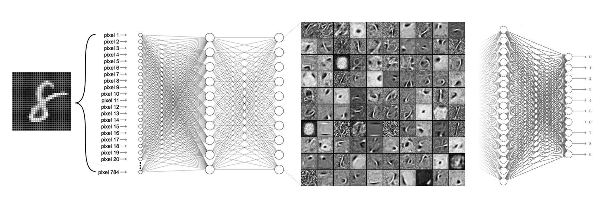
Note: The source code for this example can be found in the train.php file in project root.

Extracting the Data

The MNIST dataset comes to us in the form of 60,000 training and 10,000 testing images organized into subfolders where the folder name is the human-annotated label given to the sample. We'll use the imagecreatefrompng() function from the GD library to load the images into our script and assign them a label based on the subfolder they are in.

$samples = $labels = [];

for ($label = 0; $label < 10; $label++) {
    foreach (glob("training/$label/*.png") as $file) {
        $samples[] = [imagecreatefrompng($file)];
        $labels[] = "#$label";
    }
}

Then, we can instantiate a new Labeled dataset object from the samples and labels using the standard constructor.

use Rubix\ML\Datasets\Labeled;

$dataset = new Labeled($samples, $labels);

Dataset Preparation

We're going to use a transformer Pipeline to shape the dataset into the correct format for our learner. We know that the size of each sample image in the MNIST dataset is 28 x 28 pixels, but just to make sure that future samples are always the correct input size we'll add an Image Resizer. Then, to convert the image into raw pixel data we'll use the Image Vectorizer which extracts continuous raw color channel values from the image. Since the sample images are black and white, we only need to use 1 color channel per pixel. At the end of the pipeline we'll center and scale the dataset using the Z Scale Standardizer to help speed up the convergence of the neural network.

Instantiating the Learner

Now, we'll go ahead and instantiate our Multilayer Perceptron classifier. Let's consider a neural network architecture suited for the MNIST problem consisting of 3 groups of Dense neuronal layers, followed by a ReLU activation layer, and then a mild Dropout layer to act as a regularizer. The output layer adds an additional layer of neurons with a Softmax activation making this particular network architecture 4 layers deep.

Next, we'll set the batch size to 256. The batch size is the number of samples sent through the network at a time. We'll also specify an optimizer and learning rate which determines the update step of the Gradient Descent algorithm. The Adam optimizer uses a combination of Momentum and RMS Prop to make its updates and usually converges faster than standard stochastic Gradient Descent. It uses a global learning rate to control the magnitude of the step which we'll set to 0.0001 for this example.

use Rubix\ML\PersistentModel;
use Rubix\ML\Pipeline;
use Rubix\ML\Transformers\ImageResizer;
use Rubix\ML\Transformers\ImageVectorizer;
use Rubix\ML\Transformers\ZScaleStandardizer;
use Rubix\ML\Classifiers\MultiLayerPerceptron;
use Rubix\ML\NeuralNet\Layers\Dense;
use Rubix\ML\NeuralNet\Layers\Dropout;
use Rubix\ML\NeuralNet\Layers\Activation;
use Rubix\ML\NeuralNet\ActivationFunctions\ReLU;
use Rubix\ML\NeuralNet\Optimizers\Adam;
use Rubix\ML\Persisters\Filesystem;

$estimator = new PersistentModel(
    new Pipeline([
        new ImageResizer(28, 28),
        new ImageVectorizer(true),
        new ZScaleStandardizer(),
    ], new MultiLayerPerceptron([
        new Dense(100),
        new Activation(new ReLU()),
        new Dropout(0.2),
        new Dense(100),
        new Activation(new ReLU()),
        new Dropout(0.2),
        new Dense(100),
        new Activation(new ReLU()),
        new Dropout(0.2),
    ], 256, new Adam(0.0001))),
    new Filesystem('mnist.rbx', true)
);

To allow us to save and load the model from storage, we'll wrap the entire pipeline in a Persistent Model meta-estimator. Persistent Model provides additional save() and load() methods on top of the base estimator's methods. It needs a Persister object to tell it where the model is to be stored. For our purposes, we'll use the Filesystem persister which takes a path to the model file on disk. Setting history mode to true means that the persister will keep track of every past save.

Training

To start training the neural network, call the train() method on the Estimator instance with the training set as an argument.

$estimator->train($dataset);

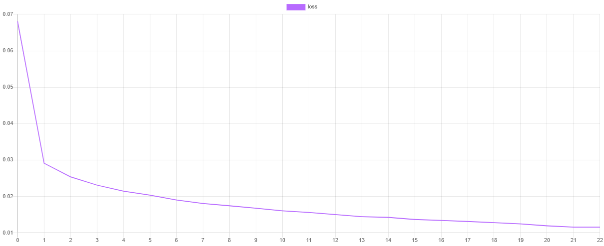
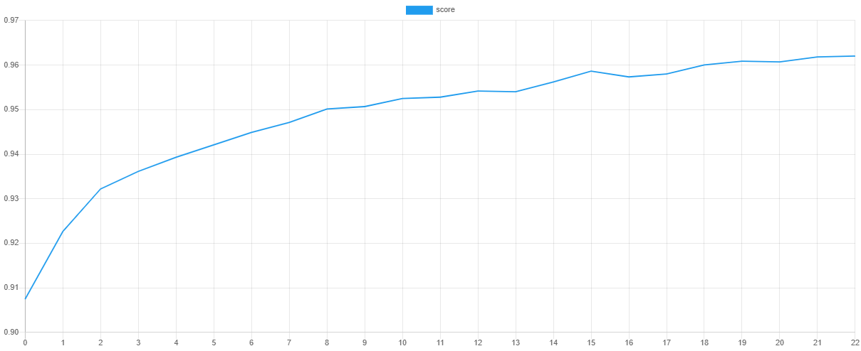
Validation Score and Loss

We can visualize the training progress at each stage by dumping the values of the loss function and validation metric after training. The steps() method will output an iterator containing the values of the default Cross Entropy cost function and the scores() method will return an array of scores from the F Beta metric.

Note: You can change the cost function and validation metric by setting them as hyper-parameters of the learner.

use Rubix\ML\Extractors\CSV;

$extractor = new CSV('progress.csv', true);

$extractor->export($estimator->steps());

Then, we can plot the values using our favorite plotting software such as Tableu or Excel. If all goes well, the value of the loss should go down as the value of the validation score goes up. Due to snapshotting, the epoch at which the validation score is highest and the loss is lowest is the point at which the values of the network parameters are taken for the final model. This prevents the network from overfitting the training data by effectively unlearning some of the noise in the dataset.

Saving

We can save the trained network by calling the save() method provided by the Persistent Model wrapper. The model will be saved in a compact serialized format such as the Native PHP serialization format or Igbinary.

$estimator->save();

Now we're ready to execute the training script from the command line.

$ php train.php

Cross Validation

Cross Validation is a technique for assessing how well the Estimator can generalize its training to an independent dataset. The goal is to identify problems such as underfitting, overfitting, or selection bias that would cause the model to perform poorly on new unseen data.

Fortunately, the MNIST dataset includes an extra 10,000 labeled images that we can use to test the model. Since we haven't used any of these samples to train the network with, we can use them to test the generalization performance of the model. To start, we'll extract the testing samples and labels from the testing folder into a Labeled dataset object.

use Rubix\ML\Datasets\Labeled;

$samples = $labels = [];

for ($label = 0; $label < 10; $label++) {
    foreach (glob("testing/$label/*.png") as $file) {
        $samples[] = [imagecreatefrompng($file)];
        $labels[] = "#$label";
    }
}

$dataset = new Labeled($samples, $labels);

Load Model from Storage

In our training script we made sure to save the model before we exited. In our validation script, we'll load the trained model from storage and use it to make predictions on the testing set. The static load() method on Persistent Model takes a Persister object pointing to the model in storage as its only argument and returns the loaded estimator instance.

use Rubix\ML\PersistentModel;
use Rubix\ML\Persisters\Filesystem;

$estimator = PersistentModel::load(new Filesystem('mnist.rbx'));

Make Predictions

Now we can use the estimator to make predictions on the testing set. The predict() method takes a dataset as input and returns an array of predictions.

$predictions = $estimator->predict($dataset);

Generating the Report

The cross validation report we'll generate is actually a combination of two reports - Multiclass Breakdown and Confusion Matrix. We'll wrap each report in an Aggregate Report to generate both reports at once under their own key.

use Rubix\ML\CrossValidation\Reports\AggregateReport;
use Rubix\ML\CrossValidation\Reports\ConfusionMatrix;
use Rubix\ML\CrossValidation\Reports\MulticlassBreakdown;

$report = new AggregateReport([
    'breakdown' => new MulticlassBreakdown(),
    'matrix' => new ConfusionMatrix(),
]);

To generate the report, pass in the predictions along with the labels from the testing set to the generate() method on the report.

$results = $report->generate($predictions, $dataset->labels());

echo $results;

Now we're ready to run the validation script from the command line.

$ php validate.php

Below is an excerpt from an example report. As you can see, our model was able to achieve 99% accuracy on the testing set.

{
    "breakdown": {
        "overall": {
            "accuracy": 0.9936867061871887,
            "accuracy_balanced": 0.9827299300164292,
            "f1_score": 0.9690024869169903,
            "precision": 0.9690931602689105,
            "recall": 0.9689771553342812,
            "specificity": 0.9964827046985771,
            "negative_predictive_value": 0.9964864183831919,
            "false_discovery_rate": 0.030906839731089673,
            "miss_rate": 0.031022844665718752,
            "fall_out": 0.003517295301422896,
            "false_omission_rate": 0.0035135816168081367,
            "threat_score": 0.939978395041131,
            "mcc": 0.9655069498416134,
            "informedness": 0.9654598600328583,
            "markedness": 0.9655795786521022,
            "true_positives": 9692,
            "true_negatives": 87228,
            "false_positives": 308,
            "false_negatives": 308,
            "cardinality": 10000
        },
        "classes": {
            "#0": {
                "accuracy": 0.9961969369924967,
                "accuracy_balanced": 0.9924488163078695,
                "f1_score": 0.9812468322351747,
                "precision": 0.9748237663645518,
                "recall": 0.9877551020408163,
                "specificity": 0.9971425305749229,
                "negative_predictive_value": 0.9986263736263736,
                "false_discovery_rate": 0.025176233635448186,
                "miss_rate": 0.01224489795918371,
                "fall_out": 0.0028574694250771415,
                "false_omission_rate": 0.0013736263736263687,
                "threat_score": 0.96318407960199,
                "informedness": 0.984897632615739,
                "markedness": 0.984897632615739,
                "mcc": 0.9791571571236778,
                "true_positives": 968,
                "true_negatives": 8724,
                "false_positives": 25,
                "false_negatives": 12,
                "cardinality": 980,
                "proportion": 0.098
            },
            "#2": {
                "accuracy": 0.9917118592039292,
                "accuracy_balanced": 0.9774202967570631,
                "f1_score": 0.960698689956332,
                "precision": 0.9620991253644315,
                "recall": 0.9593023255813954,
                "specificity": 0.9955382679327308,
                "negative_predictive_value": 0.9951967063129002,
                "false_discovery_rate": 0.03790087463556846,
                "miss_rate": 0.04069767441860461,
                "fall_out": 0.004461732067269186,
                "false_omission_rate": 0.004803293687099752,
                "threat_score": 0.9243697478991597,
                "informedness": 0.9548405935141262,
                "markedness": 0.9548405935141262,
                "mcc": 0.9560674244463004,
                "true_positives": 990,
                "true_negatives": 8702,
                "false_positives": 39,
                "false_negatives": 42,
                "cardinality": 1032,
                "proportion": 0.1032
            },
        }
    },
    "matrix": {
        "#0": {
            "#0": 968,
            "#5": 2,
            "#2": 5,
            "#9": 3,
            "#8": 3,
            "#6": 8,
            "#7": 2,
            "#3": 1,
            "#1": 0,
            "#4": 1
        },
        "#5": {
            "#0": 2,
            "#5": 859,
            "#2": 3,
            "#9": 7,
            "#8": 7,
            "#6": 5,
            "#7": 0,
            "#3": 6,
            "#1": 1,
            "#4": 0
        },
    }
}

Next Steps

Congratulations on completing the MNIST tutorial on handwritten digit recognition in Rubix ML. We highly recommend browsing the documentation to get a better feel for what the neural network subsystem can do. What other problems would deep learning be suitable for?

Original Dataset

Yann LeCun, Professor The Courant Institute of Mathematical Sciences New York University Email: yann 'at' cs.nyu.edu

Corinna Cortes, Research Scientist Google Labs, New York Email: corinna 'at' google.com

References

Y. LeCun et al. (1998). Gradient-based learning applied to document recognition.

License

The code is licensed MIT and the tutorial is licensed CC BY-NC 4.0.

rubix / mnist

Maintainers

Details