rubix / credit
An example project that predicts the risk of credit card default using a Logistic Regression classifier and a 30,000 sample dataset of credit card customers.
Maintainers
Requires
- php: >=7.4
- rubix/ml: ^2.0
README
An example Rubix ML project that predicts the probability of a customer defaulting on their credit card bill next month using a Logistic Regression estimator and a 30,000 sample dataset of credit card customers. We'll also describe the dataset using statistics and visualize it using a manifold learning technique called t-SNE.
- Difficulty: Medium
- Training time: Minutes
Installation
Clone the project locally using Composer:
$ composer create-project rubix/credit
Requirements
- PHP 7.4 or above
Recommended
- Tensor extension for faster training and inference
- 1G of system memory or more
Tutorial
Introduction
The dataset provided to us contains 30,000 labeled samples from customers of a Taiwanese credit card issuer. Our objective is to train an estimator that predicts the probability of a customer defaulting on their credit card bill the next month. Since this is a binary classification problem (will default or won't default) we can use the binary classifier Logistic Regression which implements the Probabilistic interface to make our predictions. Logistic Regression is a supervised learner that trains a linear model using an algorithm called Gradient Descent under the hood.
Note: The source code for this example can be found in the train.php file in project root.
Extracting the Data
In Rubix ML, data are passed in specialized containers called Dataset objects. We'll start by extracting the data provided in the dataset.csv file using the built-in CSV extractor and then instantiating a Labeled dataset object from it using the fromIterator() factory method.
use Rubix\ML\Datasets\Labeled;
use Rubix\ML\Extractors\CSV;

$dataset = Labeled::fromIterator(new CSV('dataset.csv', true));
Dataset Preparation
Since data types cannot be inferred from the CSV format, the entire dataset will be loaded in as strings. We'll need to convert the numeric types to their integer and floating point number counterparts before proceeding. Lucky for us, the Numeric String Converter accomplishes this task automatically.
The categorical features such as gender, education, and marital status - as well as the continuous features such as age and credit limit are now in the appropriate format. However, the Logistic Regression estimator is not compatible with categorical features directly so we'll need to One Hot Encode them to convert them into continuous ones. One hot encoding takes a categorical feature column and transforms the values into a vector of binary features where the feature that represents the active category is high (1) and all others are low (0).
In addition, it is a good practice to center and scale the dataset as it helps speed up the convergence of the Gradient Descent learning algorithm. To do that, we'll chain another transformation to the dataset called Z Scale Standardizer which standardizes the data by dividing each column over its Z score.
use Rubix\ML\Transformers\NumericStringConverter;
use Rubix\ML\Transformers\OneHotEncoder;
use Rubix\ML\Transformers\ZScaleStandardizer;

$dataset->apply(new NumericStringConverter())
    ->apply(new OneHotEncoder())
    ->apply(new ZScaleStandardizer());
We'll need to set some of the data aside so that it can be used later for testing. The reason we separate the data rather than training the learner on all of the samples is because we want to be able to test the learner on samples it has never seen before. The stratifiedSplit() method on the Dataset object fairly splits the dataset into two subsets by a user-specified ratio. For this example, we'll use 80% of the data for training and hold out 20% for testing.
[$training, $testing] = $dataset->stratifiedSplit(0.8);
Instantiating the Learner
You'll notice that Logistic Regression has a few parameters to consider. These parameters are called hyper-parameters as they have a global effect on the behavior of the algorithm during training and inference. For this example, we'll specify the first three hyper-parameters, the batch size and the Gradient Descent optimizer with its learning rate.
As previously mentioned, Logistic Regression trains using an algorithm called Gradient Descent. Specifically, it uses a form of GD called Mini-batch Gradient Descent that feeds small batches of the randomized dataset through the learner at a time. The size of the batch is determined by the batch size hyper-parameter. A small batch size typically trains faster but produces a rougher gradient for the learner to traverse. For our example, we'll pick 256 samples per batch but feel free to play with this setting on your own.
The next hyper-parameter is the GD Optimizer which controls the update step of the algorithm. Most optimizers have a global learning rate setting that allows you to control the size of each Gradient Descent step. The Step Decay optimizer gradually decreases the learning rate by a given factor every n steps from its global setting. This allows training to be fast at first and then slow down as it get closer to reaching the minima of the gradient. We'll choose to decay the learning rate every 100 steps with a starting rate of 0.01. To instantiate the learner, pass the hyper-parameters to the Logistic Regression constructor.
use Rubix\ML\Classifiers\LogisticRegression;
use Rubix\ML\NeuralNet\Optimizers\StepDecay;

$estimator = new LogisticRegression(256, new StepDecay(0.01, 100));
Setting a Logger
Since Logistic Regression implements the Verbose interface, we can hand it a PSR-3 compatible logger instance and it will log helpful information to the console during training. We'll use the Screen logger that comes built-in with Rubix ML, but feel free to choose any great PHP logger such as Monolog or Analog to do the job as well.
use Rubix\ML\Other\Loggers\Screen;

$estimator->setLogger(new Screen());
Training
Now, you are ready to train the learner by passing the training set that we created earlier to the train() method on the learner instance.
$estimator->train($dataset);
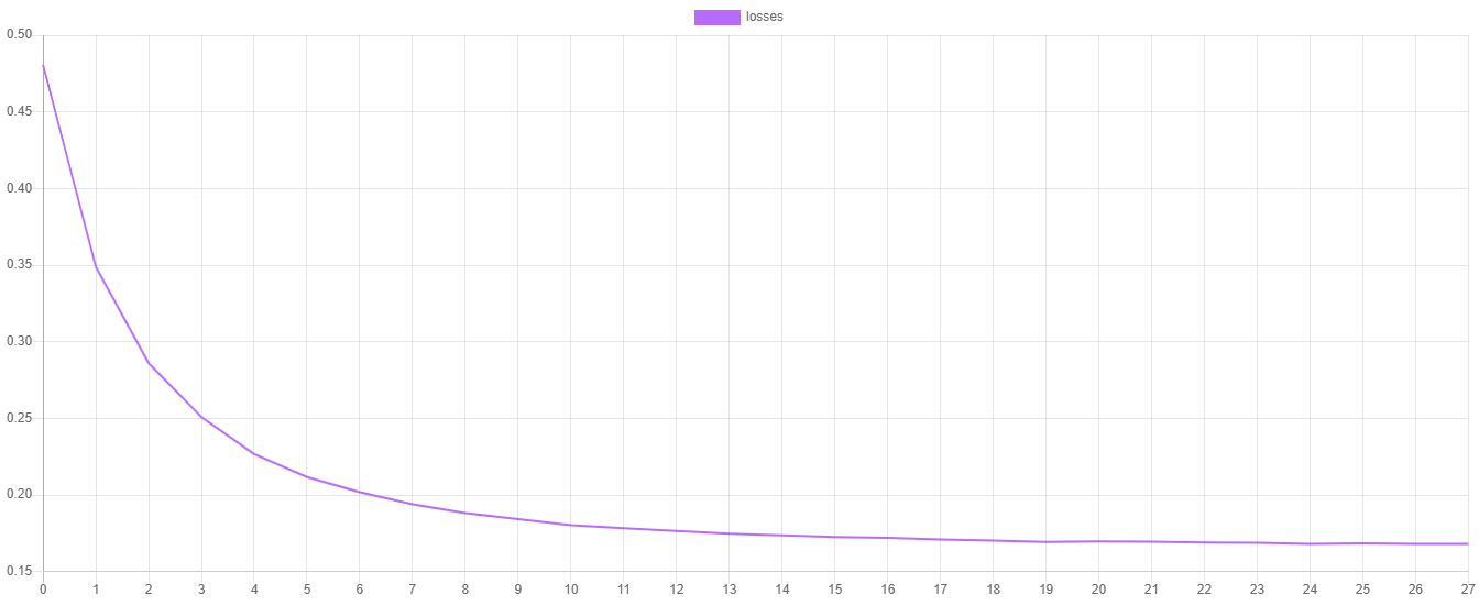
Training Loss
The steps() method on Logistic Regression outputs the value of the Cross Entropy cost function at each epoch from the last training session. You can plot those values by dumping them to a CSV file and then importing them into your favorite plotting software such as Plotly or Tableau.
use Rubix\ML\Extractors\CSV;

$extractor = new CSV('progress.csv', true);

$extractor->export($estimator->steps());
You'll notice that the loss should be decreasing at each epoch and changes in the loss value should get smaller the closer the learner is to converging on the minimum of the cost function.
Cross Validation
Once the learner has been trained, the next step is to determine if the final model can generalize well to the real world. For this process, we'll need the testing data that we set aside earlier. We'll go ahead and generate two reports that compare the predictions outputted by the estimator with the ground truth labels from the testing set.
The Multiclass Breakdown report gives us detailed metrics (Accuracy, F1 Score, MCC) about the model's performance at the class level. In addition, Confusion Matrix is a table that compares the number of predictions for a particular class with the actual ground truth. We can wrap both of these reports in an Aggregate Report to generate them both at the same time.
use Rubix\ML\CrossValidation\Reports\AggregateReport;
use Rubix\ML\CrossValidation\Reports\MulticlassBreakdown;
use Rubix\ML\CrossValidation\Reports\ConfusionMatrix;

$report = new AggregateReport([
    new MulticlassBreakdown(),
    new ConfusionMatrix(),
]);
To generate the predictions for the report, call the predict() method on the estimator with the testing set.
$predictions = $estimator->predict($testing);
Then, generate the report with the predictions and the labels by calling the generate() method on the report instance.
$results = $report->generate($predictions, $testing->labels());
Now we're ready to execute the training script and view the validation results.
$ php train.php
The output of the report should look something like the output below. In this example, our classifier is 83% accurate with an F1 score of 0.69. In addition, the confusion matrix table shows that for every time we predicted yes we were correct 471 times and incorrect 170 times.
[
    {
        "overall": {
            "accuracy": 0.8288618563572738,
            "precision": 0.7874506659370852,
            "recall": 0.6591447375205939,
            "specificity": 0.6591447375205939,
            "negative_predictive_value": 0.7874506659370852,
            "false_discovery_rate": 0.21254933406291476,
            "miss_rate": 0.3408552624794061,
            "fall_out": 0.3408552624794061,
            "false_omission_rate": 0.21254933406291476,
            "f1_score": 0.6880266172924424,
            "mcc": 0.42776751059741475,
            "informedness": 0.31828947504118776,
            "markedness": 0.5749013318741705,
            "true_positives": 4974,
            "true_negatives": 4974,
            "false_positives": 1027,
            "false_negatives": 1027,
            "cardinality": 6001
        },
        "classes": {
            "yes": {
                "accuracy": 0.8288618563572738,
                "precision": 0.734789391575663,
                "recall": 0.3546686746987952,
                "specificity": 0.9636208003423925,
                "negative_predictive_value": 0.8401119402985074,
                "false_discovery_rate": 0.26521060842433697,
                "miss_rate": 0.6453313253012047,
                "fall_out": 0.0363791996576075,
                "false_omission_rate": 0.15988805970149256,
                "f1_score": 0.47841543930929414,
                "informedness": 0.31828947504118776,
                "markedness": 0.5749013318741705,
                "mcc": 0.42776751059741475,
                "true_positives": 471,
                "true_negatives": 4503,
                "false_positives": 170,
                "false_negatives": 857,
                "cardinality": 1328,
                "density": 0.22129645059156808
            },
            "no": {
                "accuracy": 0.8288618563572738,
                "precision": 0.8401119402985074,
                "recall": 0.9636208003423925,
                "specificity": 0.3546686746987952,
                "negative_predictive_value": 0.734789391575663,
                "false_discovery_rate": 0.15988805970149256,
                "miss_rate": 0.0363791996576075,
                "fall_out": 0.6453313253012047,
                "false_omission_rate": 0.26521060842433697,
                "f1_score": 0.8976377952755906,
                "informedness": 0.31828947504118776,
                "markedness": 0.5749013318741705,
                "mcc": 0.42776751059741475,
                "true_positives": 4503,
                "true_negatives": 471,
                "false_positives": 857,
                "false_negatives": 170,
                "cardinality": 4673,
                "density": 0.7787035494084319
            }
        }
    },
    {
        "yes": {
            "yes": 471,
            "no": 170
        },
        "no": {
            "yes": 857,
            "no": 4503
        }
    }
]
Exploring the Dataset
Exploratory data analysis is the process of using analytical techniques such as statistic and scatterplots to obtain a better understanding of the data. In this section, we'll describe the feature columns of the credit card dataset with statistics and then plot a low dimensional embedding of the dataset to visualize its structure.
Note: The source code for this example can be found in the explore.php file in project root.
Begin by importing the credit card dataset and converting numerical strings like we did in a previous step.
use Rubix\ML\Datasets\Labeled;
use Rubix\ML\Extractors\CSV;
use Rubix\ML\Transformers\NumericStringConverter;

$dataset = Labeled::fromIterator(new CSV('dataset.csv', true))
    ->apply(new NumericStringConverter());
Describing the Dataset
The dataset object we instantiated has a describe() method that generates statistics for each feature column in the dataset. Category densities will be calculated for each categorical feature value and statistics such as mean, median, and standard deviation will be output for the continuous feature columns. The return value is a report object that can be echoed out to the terminal.
$stats = $dataset->describe();

echo $stats;
Here is the output of the first two columns in the credit card dataset. We can see that the first column credit_limit has a mean of 167,484 and the distribution of values is skewed to the left. We also know that column two gender contains two categories and that there are more females than males (60 / 40) represented in this dataset. Generate and examine the dataset stats for yourself and see if you can identify any other interesting characteristics of the dataset.
[
    {
        "type": "continuous",
        "mean": 167484.32266666667,
        "variance": 16833894533.632648,
        "std_dev": 129745.49908814814,
        "skewness": 0.9928173164822339,
        "kurtosis": 0.5359735300875466,
        "min": 10000,
        "25%": 50000,
        "median": 140000,
        "75%": 240000,
        "max": 1000000
    },
    {
        "type": "categorical",
        "num_categories": 2,
        "densities": {
            "female": 0.6037333333333333,
            "male": 0.39626666666666666
        }
    }
]
In addition, we'll save the stats to a JSON file so we can reference it later.
use Rubix\ML\Persisters\Filesystem;

$stats->toJSON()->saveTo(new Filesystem('stats.json'));
Visualizing the Dataset
The credit card dataset has 25 features and after one hot encoding it becomes 93. Thus, the vector space for this dataset is 93-dimensional. Visualizing this type of high-dimensional data with the human eye is only possible by reducing the number of dimensions to something that makes sense to plot on a chart (1 - 3 dimensions). Such dimensionality reduction is called Manifold Learning because it seeks to find a lower-dimensional manifold of the data. Here we will use a popular manifold learning algorithm called t-SNE to help us visualize the data by embedding it into only two dimensions.
We don't need the entire dataset to generate a decent embedding so we'll take 2,500 random samples from the dataset and only embed those. The head() method on the dataset object will return the first n samples and labels from the dataset in a new dataset object. Randomizing the dataset beforehand will remove the bias as to the sequence that the data was collected and inserted.
use Rubix\ML\Datasets\Labeled;

$dataset = $dataset->randomize()->head(2500);
Instantiating the Embedder
T-SNE stands for t-Distributed Stochastic Neighbor Embedding and is a powerful non-linear dimensionality reduction algorithm suited for visualizing high-dimensional datasets. The first hyper-parameter is the number of dimensions of the target embedding. Since we want to be able to plot the embedding as a 2-d scatterplot we'll set this parameter to the integer 2. The next hyper-parameter is the learning rate which controls the rate at which the embedder updates the target embedding. The last hyper-parameter we'll set is called the perplexity and can the thought of as the number of nearest neighbors to consider when computing the variance of the distribution of a sample. Refer to the documentation for a full description of the hyper-parameters.
use Rubix\ML\Embedders\TSNE;

$embedder = new TSNE(2, 20.0, 20);
Embedding the Dataset
Before we continue, we'll need to prepare the dataset for embedding since, like Logistic Regression, T-SNE is only compatible with continuous features. We can perform the necessary transformations on the dataset by passing the transformers to the apply() method on the dataset object like we did earlier in the tutorial.
use Rubix\ML\Transformers\OneHotEncoder;
use Rubix\ML\Transformers\ZScaleStandardizer;

$dataset->apply(new OneHotEncoder())
    ->apply(new ZScaleStandardizer());
Note: Centering and standardizing the data with Z Scale Standardizer or another standardizer is not always necessary, however, it just so happens that both Logistic Regression and t-SNE benefit when the data are centered and standardized.
Since an Embedder is a Transformer at heart, you can use the newly instantiated t-SNE embedder to embed the samples in a dataset using the apply() method.
$dataset->apply($embedder);
When the embedding is complete, we can save the dataset to a file so we can open it later in our favorite plotting software.
use Rubix\ML\Extractors\CSV;

$dataset->exportTo(new CSV('embedding.csv'));
Now we're ready to execute the explore script and plot the embedding using our favorite plotting software.
$ php explore.php
Here is an example of what a typical 2-dimensional embedding looks like when plotted.
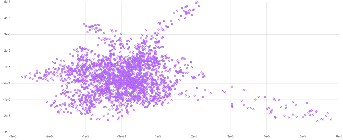
Note: Due to the stochastic nature of the t-SNE algorithm, every embedding will look a little different from the last. The important information is contained in the overall structure of the data.
Next Steps
Congratulations on completing the tutorial! The Logistic Regression estimator we just trained is able to achieve the same results as in the original paper, however, there are other estimators in Rubix ML to choose from that may perform better. Consider the same problem using an ensemble method such as AdaBoost or Random Forest as a next step.
Slide Deck
You can refer to the slide deck that accompanies this example project if you need extra help or a more in depth look at the math behind Logistic Regression, Gradient Descent, and the Cross Entropy cost function.
Original Dataset
Contact: I-Cheng Yeh
Emails: (1) icyeh '@' chu.edu.tw (2) 140910 '@' mail.tku.edu.tw
Institutions: (1) Department of Information Management, Chung Hua University, Taiwan. (2) Department of Civil Engineering, Tamkang University, Taiwan. other contact information: 886-2-26215656 ext. 3181
References
- Yeh, I. C., & Lien, C. H. (2009). The comparisons of data mining techniques for the predictive accuracy of probability of default of credit card clients. Expert Systems with Applications, 36(2), 2473-2480.
- Dua, D. and Graff, C. (2019). UCI Machine Learning Repository [http://archive.ics.uci.edu/ml]. Irvine, CA: University of California, School of Information and Computer Science.
License
The code is licensed MIT and the tutorial is licensed CC BY-NC 4.0.