README

CIFAR-10 (short for Canadian Institute For Advanced Research) is a famous dataset consisting of 60,000 32 x 32 color images in 10 classes (dog, cat, car, ship, etc.) with 6,000 images per class. In this tutorial, we'll use the CIFAR-10 dataset to train a feed forward neural network to recognize the primary object in images.

Difficulty: Hard
Training time: Hours

Installation

Clone the project locally using Composer:

$ composer create-project rubix/cifar-10

Note: Installation may take longer than usual due to the large dataset.

Requirements

PHP 7.4 or above
GD extension

Tutorial

Introduction

Computer vision is one of the most fascinating use cases for deep learning because it allows a computer to see the world that we live in. Deep learning is a subset of machine learning concerned with breaking down raw data into higher order feature representations through layered computations. Neural networks are a type of deep learning model inspired by the human nervous system that uses structured computational units called hidden layers. In the case of image recognition, the hidden layers are able to break down an image into its component parts such that the network can readily comprehend the similarities and differences among objects by their characteristic features at the final output layer. Let's get started!

Extracting the Data

The CIFAR-10 dataset comes to us in the form of 60,000 32 x 32 pixel PNG image files which we'll import as PHP resources into our project using the imagecreatefrompng() provided by the GD extension. If you do not have the extension installed, you'll need to do so before running the project script. We also use preg_replace() to extract the label from the filename of the images in the train folder.

$samples = $labels = [];

foreach (glob('train/*.png') as $file) {
    $samples[] = [imagecreatefrompng($file)];
    $labels[] = preg_replace('/[0-9]+_(.*).png/', '$1', basename($file));
}

Now, load the extracted samples and labels into a Labeled dataset object.

use Rubix\ML\Datasets\Labeled;

$dataset = new Labeled($samples, $labels);

Dataset Preparation

The images we imported in the previous step will eventually need to be converted into samples of continuous features. An Image Resizer ensures that all images have the same dimensionality, just in case. The Image Vectorizer handles extracting the red, green, and blue (RGB) intensities (0 - 255) from the images. Finally, the Z Scale Standardizer scales and centers the vectorized color channel data to a mean of 0 and a standard deviation of 1. This last step helps the network converge quicker. We'll wrap the 3 transformers in a Pipeline so we can use them again in another process after we save the model.

Instantiating the Learner

The Multilayer Perceptron classifier is a type of neural network model we'll train to recognize images in the CIFAR-10 dataset. Under the hood it uses Gradient Descent with Backpropagation to learn the weights of the network by gradually updating the signal that each neuron produces in response to an input. One of the key aspects of neural networks are the use of hidden layers that perform intermediate computations. In between Dense neuronal layers we use an Activation layer to perform a non-linear transformation of the neuron's output using a user-defined activation function. The non-linearities introduced by the activation layer are crucial for learning complex patterns within the data. For the purpose of this tutorial we'll use the ELU activation function, which is a good default but feel free to experiment with different activation functions on your own. A Dropout layer is added after the first two sets of Dense/Activation layers to act as a regularizer. Lastly, we'll add a Batch Norm layer to help the network train faster by re-normalizing the activations partway through the network.

Wrapping the learner and transformer pipeline in a Persistent Model meta-estimator allows us to save the model so we can use it in another process to make predictions.

use Rubix\ML\PersistentModel;
use Rubix\ML\Pipeline;
use Rubix\ML\Transformers\ImageResizer;
use Rubix\ML\Transformers\ImageVectorizer;
use Rubix\ML\Transformers\ZScaleStandardizer;
use Rubix\ML\Classifiers\MultilayerPerceptron;
use Rubix\ML\NeuralNet\Layers\Dense;
use Rubix\ML\NeuralNet\Layers\Activation;
use Rubix\ML\NeuralNet\Layers\Dropout;
use Rubix\ML\NeuralNet\Layers\BatchNorm;
use Rubix\ML\NeuralNet\ActivationFunctions\ELU;
use Rubix\ML\NeuralNet\Optimizers\Adam;
use Rubix\ML\Persisters\Filesystem;

$estimator = new PersistentModel(
    new Pipeline([
        new ImageResizer(32, 32),
        new ImageVectorizer(),
        new ZScaleStandardizer(),
    ], new MultilayerPerceptron([
        new Dense(200),
        new Activation(new ELU()),
        new Dropout(0.5),
        new Dense(200),
        new Activation(new ELU()),
        new Dropout(0.5),
        new Dense(100, 0.0, false),
        new BatchNorm(),
        new Activation(new ELU()),
        new Dense(100),
        new Activation(new ELU()),
        new Dense(50),
        new Activation(new ELU()),
    ], 256, new Adam(0.0005))),
    new Filesystem('cifar10.rbx', true)
);

There are a few more hyper-parameters of the MLP that we'll need to set in addition to the hidden layers. The batch size parameter is the number of samples that will be sent through the neural network at a time. We'll set this to 512. Next, the Gradient Descent optimizer and learning rate, which control the update step of the learning algorithm, will be set to Adam and 0.001 respectively. Feel free to experiment with these settings on your own.

Training

Now, pass the training dataset to the train() method to begin training the network.

$estimator->train($dataset);

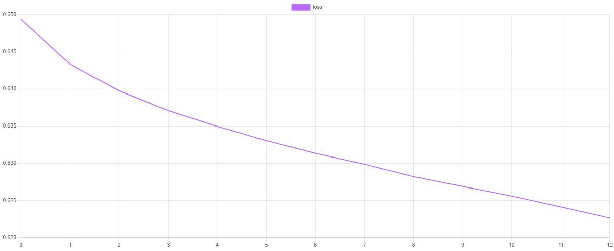
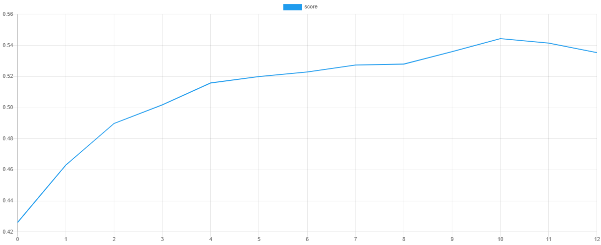
Validation Score and Loss

We can visualize the training progress at each stage by dumping the values of the loss function and validation metric after training. The steps() method will output an iterator containing the loss values of the default Cross Entropy cost function and validation scores from the default F Beta metric.

Note: You can change the cost function and validation metric by setting them as hyper-parameters of the learner.

use Rubix\ML\Extractors\CSV;

$extractor = new CSV('progress.csv', true);

$extractor->export($estimator->steps());

Then, we can plot the values using our favorite plotting software such as Tableu or Excel. If all goes well, the value of the loss should go down as the value of the validation score goes up. Due to snapshotting, the epoch at which the validation score is highest and the loss is lowest is the point at which the values of the network parameters are taken.

Saving

Before exiting the script, save the model so we can run cross validation on it in another process.

$estimator->save();

Now we're ready to execute the training script from the command line.

$ php train.php

Cross Validation

Cross validation is the process of testing a model using samples that the learner has never seen before. The goal is to be able to detect problems such as selection bias or overfitting. In addition to the training set, the CIFAR-10 dataset includes 10,000 testing samples that we'll use to score the model's generalization ability. We start by importing the testing samples and labels located in the test folder using the technique from earlier.

$samples = $labels = [];

foreach (glob('test/*.png') as $file) {
    $samples[] = [imagecreatefrompng($file)];
    $labels[] = preg_replace('/[0-9]+_(.*).png/', '$1', basename($file));
}

Instantiate a Labeled dataset object with the testing samples and labels.

use Rubix\ML\Datasets\Labeled;

$dataset = new Labeled($samples, $labels);

Load Model from Storage

Since we saved our model after training in the last section, we can load it whenever we need to use it in another process. The static load() method on the Persistent Model class takes a pre-configured Persister object pointing to the location of the model in storage as its only argument and returns the wrapped estimator in the last known saved state.

use Rubix\ML\PersistentModel;
use Rubix\ML\Persisters\Filesystem;

$estimator = PersistentModel::load(new Filesystem('cifar10.rbx'));

Make Predictions

We'll need the predictions produced by the MLP on the testing set to pass to a report generator along with the ground-truth class labels. To return an array of predictions, pass the testing set to the predict() method on the estimator.

$predictions = $estimator->predict($dataset);

Generate Reports

The Multiclass Breakdown and Confusion Matrix are cross validation reports that show performance of the model on a class by class basis. We'll wrap them both in an Aggregate Report and pass our predictions along with the ground-truth labels from the testing set to the generate() method to generate both reports at once.

use Rubix\ML\CrossValidation\Reports\AggregateReport;
use Rubix\ML\CrossValidation\Reports\ConfusionMatrix;
use Rubix\ML\CrossValidation\Reports\MulticlassBreakdown;

$report = new AggregateReport([
    new MulticlassBreakdown(),
    new ConfusionMatrix(),
]);

$results = $report->generate($predictions, $dataset->labels());

To run the validation script, enter the following command at the command prompt.

$ php validate.php

Take a look at the results to see how the model performed on inference. Below is an excerpt of a multiclass breakdown report showing the overall performance. As you can see, the model does a fair job at recognizing the objects in the images, however there is room for improvement.

"overall": {
    "accuracy": 0.8538682791748626,
    "precision": 0.5467567594653738,
    "recall": 0.5372000000000001,
    "specificity": 0.9134813190242806,
    "negative_predictive_value": 0.9138360056175517,
    "false_discovery_rate": 0.4532432405346262,
    "miss_rate": 0.46280000000000004,
    "fall_out": 0.08651868097571924,
    "false_omission_rate": 0.08616399438244826,
    "f1_score": 0.5322032931908443,
    "mcc": 0.4528826530026047,
    "informedness": 0.4506813190242807,
    "markedness": 0.46059276508292557,
    "true_positives": 5372,
    "true_negatives": 48348,
    "false_positives": 4628,
    "false_negatives": 4628,
    "cardinality": 10000,
    "density": 1
},

This excerpt from the confusion matrix shows that the estimator does a good job identifying automobiles but sometimes confuses them for trucks, which makes sense since they are similar in many ways.

    "automobile": {
        "cat": 14,
        "dog": 6,
        "airplane": 14,
        "ship": 37,
        "deer": 4,
        "automobile": 603,
        "frog": 9,
        "horse": 10,
        "bird": 12,
        "truck": 130
    },

Next Steps

Congratulations on finishing the CIFAR-10 tutorial using Rubix ML! Now is your chance to experiment with other network architectures, activation functions, and learning rates on your own. Try adding additional hidden layers to deepen the network and add flexibility to the model. Is a fully-connected network the best architecture for this problem? Are there other network architectures that can use the spatial information of the images?

Original Dataset

Creator: Alex Krizhevsky Email: akrizhevsky '@' gmail.com

References

[1] A. Krizhevsky. (2009). Learning Multiple Layers of Features from Tiny Images.

License

The code is licensed MIT and the tutorial is licensed CC BY-NC 4.0.

rubix / cifar-10

Maintainers

Details