rubix / churn
Maintainers
Requires
- php: >=7.4
- rubix/ml: ^2.3
This package is auto-updated.
Last update: 2026-06-25 21:42:07 UTC
README
Machine Learning is a paradigm shift from traditional programming because it allows the software itself to modify its programming through training and data. For this reason, you can think of Machine Learning as “programming with data.” Integrating ML into your project is therefore a practice of merging logic written by developers with logic that was learned by a Machine Learning algorithm. Today, we’ll talk about how you can start integrating Machine Learning models into your PHP projects using the open-source Rubix ML library. We’ll formulate the problem of customer churn prediction, train a model to identify what an unhappy customer looks like, and then use that model to detect the unhappy customers within our database.
- Difficulty: Moderate
- Training time: Seconds
Installation
Clone the project locally using Composer:
$ composer create-project rubix/churn
Requirements
- PHP 7.4 or above
Tutorial
Introduction
Let’s start by introducing the problem of predicting customer churn. Churn rate is the rate at which customers discontinue use of a product or service over a period of time. If we could predict which of our customers are most likely to leave, then we could take action to try to repair the relationship before they are gone. But, how do we as developers encode the ruleset i.e. the “business logic” that determines what an unhappy customer looks like?
Imagine that you are a developer working at a telecommunications company tasked with optimizing customer churn. One thing you could do is ask the customer service department what customers say about the service. You might learn that our customers who live in a certain region were more likely to complain of slow Internet speed and discontinue their service. You might also learn that older customers were really happy with the streaming TV and movie selection and were therefore more likely to hold onto their subscription. You could start by encoding these rules out by hand, but this quickly becomes overwhelming when you consider all the different factors that contribute to customer satisfaction. Instead, we can feed samples of both satisfied and unsatisfied customers through a learning algorithm and have the learner learn the rules automatically. Then, we can take that model and use it to make predictions about the customers in our database.
Preparing the Dataset
Before training the model, we need to gather the samples of satisfied and unsatisfied customers and label them accordingly. Then, we'll determine which features of a customer are beneficial in determining whether or not a customer will churn. For example, service region and the number of times the customer called for tech support are probably good features to include in the dataset, but features such as eye color and whether or not the customer has a back yard or not may be counterproductive to include them. In the example below, we'll load the samples from the provided example dataset using the CSV extractor and then select a subset of the features using the ColumnPicker. In Rubix ML, Extractors are iterators that stream data from storage into memory and can be wrapped by other iterators to modify the data in-flight. Note that we've included the label for each sample as the last column of the data table as is the convention.
use Rubix\ML\Extractors\CSV;
use Rubix\ML\Extractors\ColumnPicker;

$extractor = new ColumnPicker(new CSV('dataset.csv', true), [
    'Gender', 'SeniorCitizen', 'Partner', 'Dependents', 'MonthsInService', 'Phone',
    'MultipleLines', 'InternetService', 'OnlineSecurity', 'OnlineBackup', 'DeviceProtection',
    'TechSupport', 'TV', 'Movies', 'Contract', 'PaperlessBilling', 'PaymentMethod',
    'MonthlyCharges', 'TotalCharges', 'Region', 'Churn',
]);
In Rubix ML, dataset objects provide a high-level API that allow you to process the samples and create subsets among other things. Next, we'll instantiate a Labeled dataset object by passing the extractor object to the static fromIterator() method.
use Rubix\ML\Datasets\Labeled;

$dataset = Labeled::fromIterator($extractor);
The next thing we'll do is create two subsets of the dataset to be used for training and testing. The training set will be used by Naive Bayes to learn a model and the testing set will be used to gauge the model's accuracy after training. Randomizing the samples before creating the subsets helps reduce potential biases introduced by the data collection method. Stratifying the samples by label ensures that the class proportions are maintained in both subsets. In the example below, we'll put 80% of the labeled samples into the training set and use the remaining 20% for validation later using the randomized stratified splitting method.
Note: The reason we use different samples to train the model than to validate it is because we want to test the learner on samples it has never seen before.
[$training, $testing] = $dataset->randomize()->stratifiedSplit(0.8);
Training the Model
Naive Bayes is an algorithm that uses counting and Bayes' Theorem to derive the conditional probabilities of a label given a sample consisting of only categorical features. The term “naive” is in reference to the algorithm’s feature independence assumption. It's naive because, in the real world, most features have interactions. In practice however, this assumption turns out not to be such a big problem.
To instantiate our Naive Bayes estimator we need to call the constructor with a set of parameters (called "hyper-parameters") that will control how the learner behaves. The current implementation of Naive Bayes has two hyper-parameters that we need to be aware of. The priors argument allows the user to specify the class prior probabilities (i.e. the probability that a particular class will be the outcome if chosen randomly) instead of the default which is to calculate the prior probabilities from the training set. For example, if we know that our average churn rate is about 5% in real life, then we can specify that as the "Yes" class's prior probability and Naive Bayes will make predictions accordingly. The second hyper-parameter is the smoothing parameter which controls the amount of Laplacian smoothing added to the conditional probabilities of each feature calculated during training. Smoothing is a form of regularization that prevents the model from being overconfident especially when the number of training samples is low. For the purposes of this example, we'll leave the smoothing parameter set at the default value of 1.0 but feel free to experiment with these settings on your own to see how they effect the accuracy of the model.
use Rubix\ML\Classifiers\NaiveBayes;

$estimator = new NaiveBayes([
    "Yes" => 0.05,
    "No" => 0.95,
]);
In the example dataset, MonthsInService, MonthlyCharges, and TotalCharges features all have numerical values. Since all values in CSV format are interpreted as strings by default, we'll need to apply a preprocessing step that converts the numeric strings (ex. "42") in the dataset to their integer and floating point representations. For this, we'll apply a stateless Transformer called Numeric String Converter to convert all the values in the first preprocessing step. Since Naive Bayes is only compatible with categorical features however, in the next step we'll also apply Interval Discretizer to derive 3 discrete categories from the aforementioned numerical features. In the context of MonthsInService, you can think of this transformation as converting the number of months to one of three equally proportional levels - "short", "medium", or "long."
We'll wrap the entire series of transformations as well as the Naive Bayes estimator in a Pipeline meta-Estimator to automatically fit and preprocess the dataset before training or inference. Fitting a transformer is analogous to training a learner and by wrapping both the transformers and estimator we can save both the transformer fittings as well as the model parameters as one atomic object.
use Rubix\ML\Pipeline;
use Rubix\ML\Transformers\NumericStringConverter;
use Rubix\ML\Transformers\IntervalDiscretizer;

$estimator = new Pipeline([
    new NumericStringConverter(),
    new IntervalDiscretizer(3, true),
], $estimator);
Now we're ready to fit the transformers and train the model by passing the training dataset to the newly instantiated Pipeline meta-Estimator.
$estimator->train($training);
We can verify that the learner has been trained by calling the trained() method on the Estimator interface.
var_dump($estimator->trained());
bool(true)
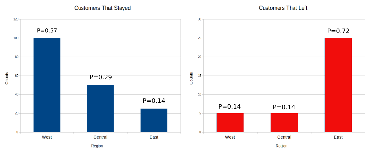
To better understand what happened when we called the train() method let's peak under the hood of the Naive Bayes algorithm for a brief moment. The first thing the algorithm did was build a histogram for each feature for a particular class outcome by counting the number of times a category appeared in the training data. The algorithm then calculates the conditional probabilities for each category from the histogram by dividing the counts over the sample size. The algorithm repeats this process for every categorical feature in the dataset. Later, we'll demonstrate how these conditional probabilities are combined to produce the overall probability of a class outcome. In the example below, we see the histograms of the Region feature. Notice that customer with service in the East region were more likely to churn than other regions.
Making Test Predictions
We're going to need to generate some test predictions for the validation step in the process. The operation of making predictions is referred to as "inference" in Machine Learning terms because it involves taking an unlabeled sample and inferring its label. To return a set of predictions, pass the testing dataset to the predict() method on the estimator after it has been trained.
$predictions = $estimator->predict($testing);
We can view the class predictions by outputting them to the terminal like in the example below.
print_r($predictions);
Array
(
    [0] => No
    [1] => No
    [2] => No
    [3] => Yes
    [4] => No
)
Under the hood, the Naive Bayes algorithm combines the prior probability with the conditional probabilities of the unknown sample for each possible class and then predicts the class with the highest posterior probability. The following formula denotes the decision function that Naive Bayes uses to make a class prediction where p(Ck) is the class prior probability given as a hyper-parameter in this case and p(xi | Ck) is the conditional probability of class Ck given feature xi that was calculated during training.
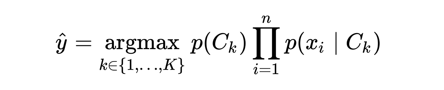
Although this formula accurately represents the high-level Naive Bayes decision function, the actual calculation in Rubix ML is done in logarithmic space. Since very low probabilities have a tendency to become unstable when multiplied together, log probabilities offer greater numerical stability by converting the products in the original formula to summations.
Validating the Model
With the test predictions and their ground-truth labels in hand, we can now turn our focus to validating the model using the "holdout" technique. The process we use to determine generalization performance is called cross-validation and the holdout technique is one of the most straightforward approaches. The upside to this method is that it's quick and only requires training one model to produce a meaningful validation score. However, the downside to this technique is that, since the validation score for the model is only calculated from a portion of the samples, it has less coverage than methods that train multiple models and test them on different samples each time. In the next example, we're are going to generate a report from the held out testing data that contains detailed metrics for us to evaluate the accuracy of the model.
We'll instantiate a Multiclass Breakdown and Confusion Matrix report generator and wrap them in an Aggregate Report so they can be generated at the same time. Multiclass Breakdown is a detailed report containing scores for a multitude of metrics including Accuracy, Precision, Recall, F-1 Score, and more on an overall and per-class basis. Confusion Matrix is a table that pairs the predictions counts on one axis with their ground-truth counts on the other. Counting each pair gives us a sense for which classes the estimator might be "confusing" another class for.
use Rubix\ML\CrossValidation\Reports\AggregateReport;
use Rubix\ML\CrossValidation\Reports\ConfusionMatrix;
use Rubix\ML\CrossValidation\Reports\MulticlassBreakdown;

$reportGenerator = new AggregateReport([
    new MulticlassBreakdown(),
    new ConfusionMatrix(),
]);
To create the report object call the generate() method on the report generator with the predictions we generated from the testing set and ground-truth labels as arguments.
$report = $reportGenerator->generate($predictions, $testing->labels());
Since the Report object implements the Stringable interface, we can output the report by echoing it out directly to the terminal. The example below illustrates a typical report for this classifier and dataset. You'll notice that Naive Bayes did a pretty good job at distinguishing the churned customers with an accuracy of about 78%.
echo $report
[
    {
        "overall": {
            "accuracy": 0.7806955287437899,
            "balanced accuracy": 0.7405835852127411,
            "f1 score": 0.7301102604109521,
            "precision": 0.7226865136298422,
            "recall": 0.7405835852127411,
            "specificity": 0.7405835852127411,
            "negative predictive value": 0.7226865136298422,
            "false discovery rate": 0.27731348637015785,
            "miss rate": 0.2594164147872588,
            "fall out": 0.2594164147872588,
            "false omission rate": 0.27731348637015785,
            "mcc": 0.4629242695197278,
            "informedness": 0.4811671704254823,
            "markedness": 0.4453730272596843,
            "true positives": 1100,
            "true negatives": 1100,
            "false positives": 309,
            "false negatives": 309,
            "cardinality": 1409
        },
        "classes": {
            "No": {
                "accuracy": 0.7806955287437899,
                "balanced accuracy": 0.7405835852127411,
                "f1 score": 0.8469539375928679,
                "precision": 0.8689024390243902,
                "recall": 0.8260869565217391,
                "specificity": 0.6550802139037433,
                "negative predictive value": 0.5764705882352941,
                "false discovery rate": 0.13109756097560976,
                "miss rate": 0.17391304347826086,
                "fall out": 0.34491978609625673,
                "false omission rate": 0.42352941176470593,
                "informedness": 0.4811671704254823,
                "markedness": 0.4453730272596843,
                "mcc": 0.4629242695197278,
                "true positives": 855,
                "true negatives": 245,
                "false positives": 129,
                "false negatives": 180,
                "cardinality": 1035,
                "proportion": 0.7345635202271115
            },
            "Yes": {
                "accuracy": 0.7806955287437899,
                "balanced accuracy": 0.7405835852127411,
                "f1 score": 0.6132665832290363,
                "precision": 0.5764705882352941,
                "recall": 0.6550802139037433,
                "specificity": 0.8260869565217391,
                "negative predictive value": 0.8689024390243902,
                "false discovery rate": 0.42352941176470593,
                "miss rate": 0.34491978609625673,
                "fall out": 0.17391304347826086,
                "false omission rate": 0.13109756097560976,
                "informedness": 0.4811671704254823,
                "markedness": 0.4453730272596843,
                "mcc": 0.4629242695197278,
                "true positives": 245,
                "true negatives": 855,
                "false positives": 180,
                "false negatives": 129,
                "cardinality": 374,
                "proportion": 0.2654364797728886
            }
        }
    },
    {
        "No": {
            "No": 855,
            "Yes": 129
        },
        "Yes": {
            "No": 180,
            "Yes": 245
        }
    }
]
We can also save the report to share with our colleagues or look at later. To save the report, call the saveTo() method on the Encoding object that is returned by calling the toJSON() method on the Report object. In this example, we'll use the Filesystem Persister to save the report to a file named report.json.
use Rubix\ML\Persisters\Filesystem;

$report->toJSON()->saveTo(new Filesystem('report.json'));
Saving the Model
We'll also save the Pipeline estimator so that we can use it in another process to predict the customers in our database. Rubix ML provides another meta-Estimator called Persistent Model that wraps a Persistable estimator and provides methods for saving and loading the model parameters from storage. In the example below we'll wrap our Pipeline object with Persistent Model and save it to the filesystem using the default RBX serializer. RBX is a proprietary format that builds on PHP's native serialization by adding compression, integrity checking, and version compatibility detection. You could also use the standard PHP Native serializer if you wanted to.
use Rubix\ML\PersistentModel;
use Rubix\ML\Persisters\Filesystem;

$estimator = new PersistentModel($estimator, new Filesystem('model.rbx'));

$estimator->save();
Going Into Production
In practice, we'd probably spend some more time iterating over training and cross-validation in an effort to fine-tune the dataset and hyper-parameters. For the next part of this tutorial, we'll assume that we're fine with the model performance so far and we're ready to put it into production.
First, we need to make the choice between doing real-time inference or caching the predictions. For this problem, it makes a lot of sense to generate predictions for all our customers at the same time and then storing the prediction in the database alongside the customer's data. Then, we could periodically predict the new customers and update the existing customers using a script that runs in the background of our application. The nice thing about this design is that we don't need to keep the model loaded into memory. However, if you need the prediction for new customers instantly or if you have a quickly evolving model, you may want to consider doing inference in real time. See the Server package for an example of how to do this in a performant way using asynchronous PHP and a long-running process.
We're going to start a new script for predicting the label of the customers in our database. For demonstration, we've provided an example Sqlite database with over 2000 customers. Let's load the samples from the database and use our saved model to predict the at-risk customers. The SQL Table extractor is an iterator that iterates over an entire database table. In the next example, we'll pass a PDO object referencing our Sqlite database to the SQL Table extractor's constructor along with the name of the table we want to iterate over.
use Rubix\ML\Extractors\SqlTable;
use PDO;

$connection = new PDO('sqlite:database.sqlite');

$extractor = new SqlTable($connection, 'customers');
If we didn't want to load all the customers in our database, we could wrap the extractor within the standard PHP Limit Iterator to specify an offset and a limit.
$extractor = new LimitIterator($extractor->getIterator(), 0, 100);
As we did with the training and validation sets, we'll instantiate a Column Picker to select the features from the database to input to the estimator. We'll also include the Id column which we'll use later when we update the database with the predictions.
$extractor = new ColumnPicker($extractor, [
    'Id', 'Gender', 'SeniorCitizen', 'Partner', 'Dependents', 'MonthsInService', 'Phone',
    'MultipleLines', 'InternetService', 'OnlineSecurity', 'OnlineBackup', 'DeviceProtection',
    'TechSupport', 'TV', 'Movies', 'Contract', 'PaperlessBilling', 'PaymentMethod',
    'MonthlyCharges', 'TotalCharges', 'Region',
]);
Now, instantiate an Unlabeled dataset object by calling the fromIterator() method with the extractor as an argument.
$dataset = Unlabeled::fromIterator($extractor);
To return the customer ids for every sample in the dataset, call the feature() method with the column offset of 0. Avoid feeding the customer Id to the estimator by dropping the it from the dataset.
$ids = $dataset->feature(0);

$dataset->dropFeature(0);
We're almost there! Now, lets load the Pipeline estimator we saved earlier into memory by calling the load() method on the Persistent Model meta-Estimator class with a Filesystem persister pointing to the path of the model file in storage as an argument. Note that you may have to supply an option Serializer if the default one wasn't used. Once loaded from storage, the estimator is ready to go in the same state that it was saved in.
$estimator = PersistentModel::load(new Filesystem('model.rbx'));
Finally, return the predictions for the customers in the database by passing the inference set to the predict() method on the Pipeline meta-Estimator. The predictions will be returned in the same order as the samples we loaded from the database.
$predictions = $estimator->predict($dataset);
We'll use the same PDO connection object from before to prepare a SQL statement to update the customer. From here, we can loop through the predictions and update the corresponding rows in the database.
$statement = $connection->prepare("UPDATE customers SET churn=? WHERE id=?");

foreach ($predictions as $i => $prediction) {
    $statement->execute([$prediction, $ids[$i]]);
}
Voila! You've identified the customers that may be at risk of churning. Let's take a moment to recap. Remember we loaded a training dataset that had been labeled by our customer service department as either churning or not churning. Then we used that dataset to train a Naive Bayes classifier to predict the churn rate of the customers in our database. Lastly, we stored those predictions in the database so we could use them later within our app. Nice work! For further learning you may want to consider ...
- Training with a different subset of the features. Are some features more predictive than others?
- How does different prior probabilities and the smoothing hyper-parameter effect the predictions?
- Swapping Naive Bayes for another classifier that is compatible with categorical features such as Random Forest or Logit Boost.
Original Dataset
https://github.com/codebrain001/customer-churn-prediction
License
The code is licensed MIT and the tutorial is licensed CC BY-NC 4.0.